Support Vector Machines(SVMs)

SVMs is a powerful supervised learning algorithm primarily used for classification tasks and works well when data is linearly separable. It can be used for regression tasks as well.

SVMs are based on the concept of support vectors. SVMs are the data points that lies close to the decision boundary (the hyperplane). Support vectors determine the position and orientation of the hyperplane.

Margin is the distance between support vectors and decision boundary for each class. SVMs aims to maximize the margin to build more generalized and robust models.

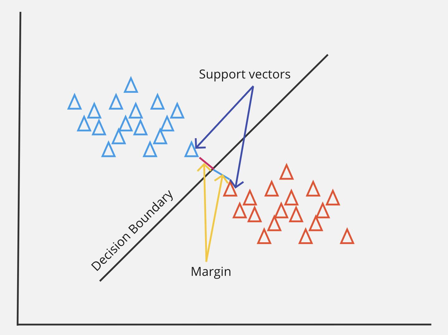
In 2-D coordinates, decision boundary is a line.
In 3-D coordinates, decision boundary is a plane.
In n-D coordinates, decision boundary is a hyperplane.
Note : Decision boundary is a region of data space that separates two or more classes.

The equation of hyperplane in n-dimensional space is represented as:

$$w.x + b = 0$$

where; w = weight vector , x = input vector , b = bias term.

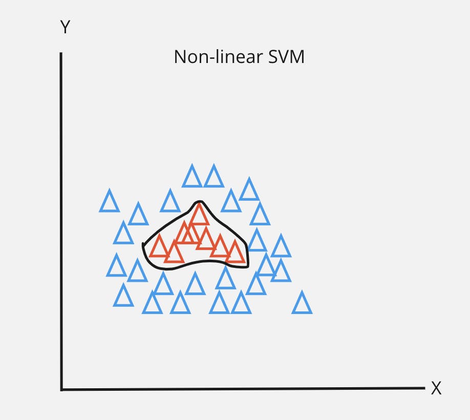
SVMs can handle non-linear relationships through kernel trick.
The idea is to map the input data points into higher dimensional space without explicitly calculating the transformation.

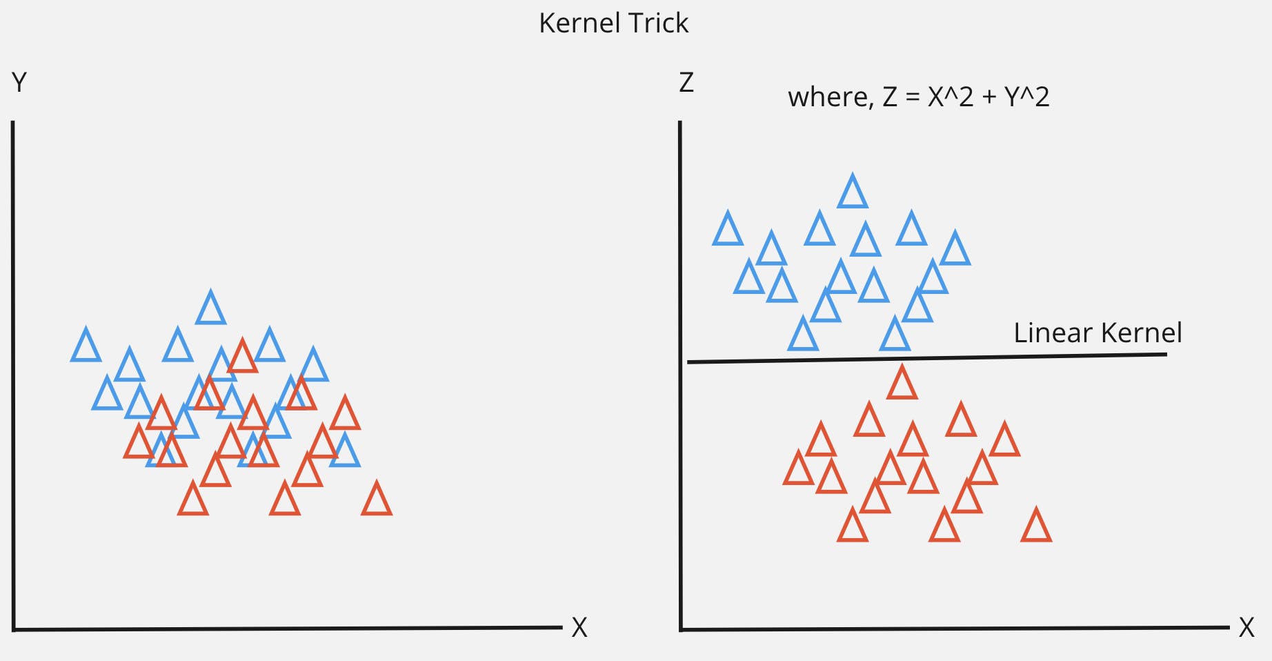
The kernel function computes the dot product of the transformed data points in higher dimensional space.

Common kernel functions are:
Linear kernel:

$$K(x i ​ ,x j ​ )=x i ​ ⋅x j ​$$

Polynomial kernel:

$$K(x i ​ ,x j ​ )=(x i ​ ⋅x j ​ +c) d $$

Advantages:

• Effective in higher dimensional spaces.

• Robust against overfitting.

• Suitable for both linear and non-linear classifications.

Example use cases:

1. Determining the sentiment expressed in the piece of text (i.e. positive, negative or neutral)

2. Identify and verify the identity of a person based on facial features in images or video.

Random Forests

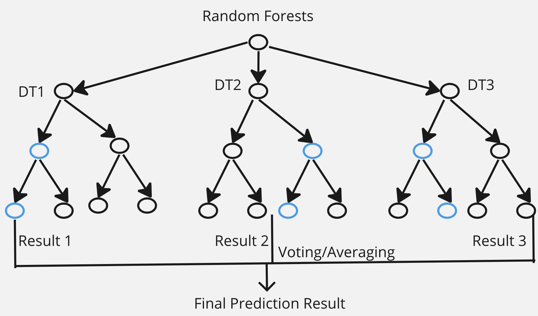
Random Forest is an ensemble learning method that builds multiple decision trees during training.

Each tree is constructed using a random subset of the training data and a random subset of features.

The final prediction is made by aggregating the predictions of individual trees (majority vote for classification, average for regression).

Advantages:

• Robust and less prone to overfitting compared to individual decision trees.

• Provides feature importance scores.

• Handles high-dimensional data well.

Example Use Cases:

1. Fraud detection in finance.

2. Remote sensing for land cover classification.

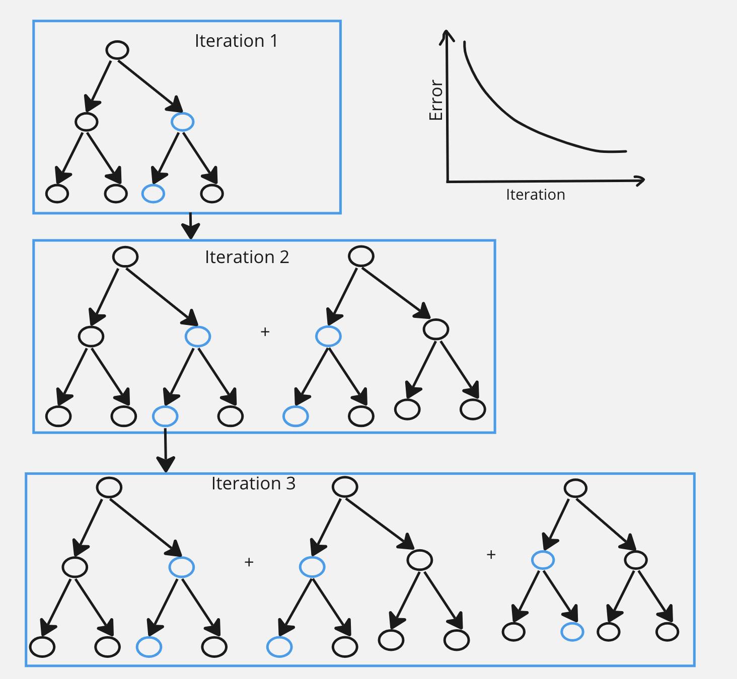
Gradient Boosting

Gradient Boosting (Gradient Boosting Machines i.e. GBMs) is an ensemble technique that builds a series of weak learners (typically decision trees) sequentially.

GBMs iteratively corrects errors made by the combined model using weak learners.

At each iteration, residuals is calculated as:

$$Residuals = y - predictions_{of PreviousIteration}$$

A new weak learner is fitted to the residuals of the combined model.

The goal is to minimize a specified loss function, which measures the difference between predicted values and true target values.

Each tree corrects the errors of the previous one, emphasizing misclassified instances.

Combines the predictions of all trees to make the final prediction.

Advantages:

• Handles both numerical and categorical data.

• Provides high accuracy and is robust.

Example Use Cases:

1. Kaggle competitions and data science competitions.

2. Click-through rate prediction in online advertising.

3. Anomaly detection in cybersecurity.

Conclusion

These are some important and powerful ML algorithms. They excel in extracting meaningful patterns and relationships, enabling more accurate predictions and informed decision-making. Each algorithm has its own strengths and weakness. So, it is essential to tailor the approach of algorithm according to the problem you are solving.